3. Research Methodology
3.1. Proposed Method
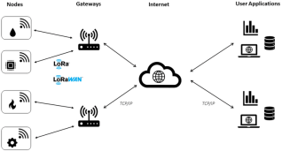
The research methodology focuses on designing and implementing a reinforcement learning (RL)-based scheduling algorithm for reliable data delivery in LoRaWAN networks. It adopts a design science research (DSR) approach, which emphasizes systematic development and evaluation of practical solutions to address inefficiencies in existing task scheduling mechanisms. The methodology begins with a detailed description of the research design, which emphasizes the need for a task scheduling algorithm that can effectively manage resources in dynamic environments. The study identifies the limitations of existing scheduling methods in LoRaWAN networks, particularly their inability to meet the QoS demands of modern IoT applications. To address these challenges, the research proposes a reinforcement learning (RL) based algorithm that can adapt to varying network conditions and optimize resource allocation.
3.2. Research Design
The research employs a mixed-methods approach, combining quantitative research with design science to systematically design, develop, and assess a QoS-aware task-scheduling algorithm. This approach allows for addressing questions related to the effectiveness of the proposed algorithm in improving QoS in dynamic IoT environments.
3.3. Algorithm Design and Implementation
3.3.1. Algorithm Design
The design of the RL-based scheduling algorithm focuses on creating an intelligent agent that optimizes task scheduling in a LoRaWAN environment. Key components include defining the state space, action space, and reward function, which guide the agent's learning process to make optimal scheduling decisions based on network conditions.
1. State Space: The state space encompasses various network parameters, such as node status, channel conditions, and traffic patterns, allowing the agent to assess the current environment effectively.
2. Action Space: The action space includes possible scheduling actions, such as channel selection, task prioritization, and gateway allocation, enabling the agent to make informed decisions to enhance QoS metrics.
3. Reward Function: The reward function is designed to provide feedback to the agent based on its actions, encouraging behaviors that lead to improved QoS outcomes, such as reduced delay, increased packet delivery ratio, and minimized packet error rates.
4. Policy (π): The policy defines the strategy the agent uses to select actions based on the observed state, enabling it to balance exploration and exploitation during learning.
5. Learning Algorithm: A suitable reinforcement learning algorithm, such as Deep Q-Networks (DQN), is employed to enable the agent to learn from its experiences and improve its scheduling decisions over time.
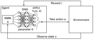
Figure 2 illustrates the architecture of a Deep Q-Network (DQN), which combines Q-learning with deep neural networks to enable reinforcement learning in complex environments. The architecture typically consists of the following key components:
1. Input Layer: This layer receives the state representation of the environment, which can include various features relevant to the task at hand. The input is often a high-dimensional vector that captures the current state of the system.
2. Hidden Layers: The DQN architecture includes multiple fully connected hidden layers (in this case, two layers) that process the input data. Each hidden layer consists of a specified number of neurons (e.g., 128), which are responsible for extracting features and learning non-linear relationships between the input state and potential actions. ReLU (Rectified Linear Unit) activation functions are commonly used to introduce non-linearity.
3. Output Layer: The output layer generates Q-values for each possible action based on the processed input state. These Q-values represent the expected future rewards for taking specific actions in the given state, allowing the agent to make informed decisions about which action to take.
4. Experience Replay: Although not explicitly shown in the architecture diagram, experience replay is an integral part of the DQN framework. It involves storing past experiences (state, action, reward, next state) in a replay memory, which is sampled during training to improve learning stability and efficiency.
The diagram shows the agent taking an action in the environment, receiving a new state and reward, and updating its policy based on the experience. This iterative process allows the agent to learn an optimal policy for maximizing rewards in the environment.
Here's a breakdown of the diagram's elements:
1) Agent: This is the decision-making entity. It receives the current state of the environment (s) and uses its policy (π) to select an action (a). The policy is typically implemented as a neural network (DNN) with parameters θ.
2) Environment: This is the external world the agent interacts with. It receives the agent's action (a) and provides the agent with a new state (s') and a reward (r).
3) State (s): The current situation or observation of the environment.
4) Action (a): The decision or move made by the agent.
5) Reward (r): A scalar value indicating the outcome of the agent's action. Positive rewards encourage behaviors, while negative rewards discourage them.
6) Policy (π): A function that maps states to actions. In DRL, it's often represented as a neural.
7) network.
a). Training Phase of the Proposed Scheduling Algorithm
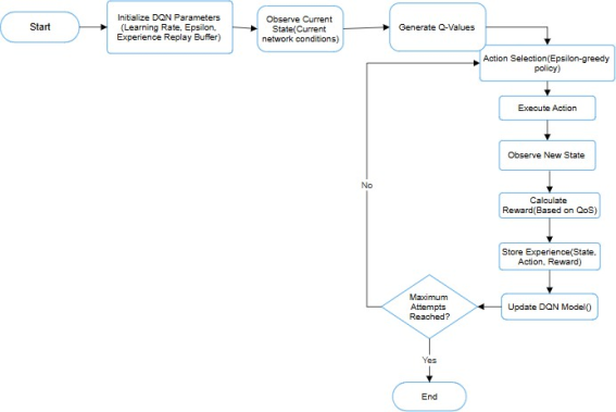
Figure 3 outlines the training phase of the proposed scheduling algorithm, which utilizes a Deep Q-Network (DQN) approach to optimize task scheduling in a LoRaWAN environment. The training phase consists of several key steps:
1. Initialization of DQN Parameters: The training process begins with the initialization of essential DQN parameters, including the learning rate, which determines how much the Q-values are updated during training; epsilon, which controls the exploration-exploitation trade-off; and the experience replay buffer, which stores past experiences to enhance training stability.
2. Observation of Current State: The agent interacts with the OpenAI Gym environment to observe the current state of the network. This state includes various parameters such as network conditions, task queue status, and other relevant metrics that influence scheduling decisions.
3. Action Selection and Execution: Based on the observed state, the agent selects an action using an epsilon-greedy policy, balancing exploration of new actions and exploitation of known rewarding actions. The selected action is then executed within the environment.
4. Reward Calculation: After executing the action, the agent receives feedback in the form of a reward, which quantifies the effectiveness of the action taken in terms of QoS metrics such as delay, throughput, and packet delivery ratio.
5. Experience Storage and Learning: The agent stores the experience (state, action, reward, next state) in the replay buffer. A mini-batch of experiences is sampled from this buffer to update the Q-values, allowing the agent to learn from past actions and improve its scheduling policy over time.
6. Iteration and Convergence: The training process continues iteratively, with the agent observing new states, selecting actions, and updating Q-values until a predefined maximum number of training iterations is reached or the performance converges to an acceptable level.
Figure 3. Training Phase of the Proposed Scheduling Algorithm.
b). The Trained Proposed Scheduling Algorithm Diagram
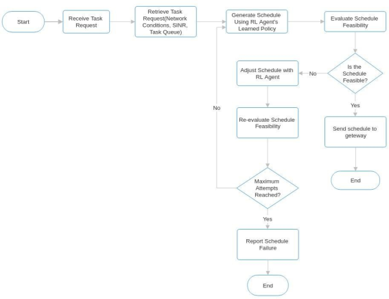
Figure 4 presents a diagram of the trained proposed scheduling algorithm, illustrating the workflow and key components involved in the task scheduling process within a LoRaWAN environment. The diagram outlines the following steps:
1. Receive Task Request: The process begins with the system receiving a new task-scheduling request, which includes critical parameters such as deadlines and network context. This initiates the scheduling cycle.
2. Retrieve Network State: The algorithm retrieves the current network state, which encompasses various factors like Signal-to-Interference-plus-Noise Ratio (SINR), existing task queue, and other relevant network conditions that influence scheduling decisions.
3. Generate Schedule: Utilizing the learned policy from the training phase, the reinforcement learning (RL) agent generates a schedule by assigning tasks to specific gateways. This assignment is optimized based on Quality of Service (QoS) metrics and the deadlines specified in the task request.
4. Evaluate Schedule Feasibility: The generated schedule is assessed for feasibility, ensuring that it meets all required constraints and QoS criteria. This step is crucial to confirm that tasks can be completed within their deadlines and adhere to the necessary QoS standards.
5. Feasibility Check: If the schedule is deemed feasible, it is sent to the relevant gateways for execution. If not, the algorithm enters an adjustment phase to refine the schedule.
6. Adjust Schedule with RL Agent: In cases where the initial schedule is infeasible, the RL agent recalibrates the task assignments to meet the QoS requirements, iteratively adjusting the schedule until it becomes feasible or the maximum number of attempts is reached.
7. Re-evaluate Schedule Feasibility: The adjusted schedule undergoes another feasibility evaluation to ensure compliance with the required constraints.
8. Final Outcome: If a feasible schedule is produced, it is transmitted to the gateways for execution. If a feasible schedule cannot be achieved within the maximum attempts, a failure report is generated, indicating that the task scheduling request could not be fulfilled.
Overall,
Figure 4 effectively illustrates the structured workflow of the trained scheduling algorithm, highlighting the interaction between task requests, network state retrieval, schedule generation, feasibility evaluation, and adjustments made by the RL agent to optimize task scheduling in a LoRaWAN network.
Figure 4. The trained proposed scheduling algorithm diagram.
3.3.2. Algorithm Implementation
The implementation of the RL-based scheduling algorithm involves translating the designed components into a functional system that operates within the simulated LoRaWAN environment. This process includes several key steps:
1. Initialization: The algorithm initializes the RL agent, setting up the state space, action space, and reward structure, along with any necessary parameters for the learning process.
2. Training Phase: The agent interacts with the environment through a reinforcement learning loop, where it observes the current state, selects actions based on its policy, receives rewards, and updates its knowledge (Q-values) to improve future decision-making.
3. Integration with Simulation: The algorithm is integrated with the network simulator (NS-3), allowing for real-time interaction with the simulated LoRaWAN network. This integration enables the agent to adapt its scheduling decisions based on dynamic network conditions and traffic patterns.
4. Evaluation: The performance of the implemented algorithm is evaluated using various QoS metrics, such as delay, packet delivery ratio, and packet error rate, to assess its effectiveness in optimizing task scheduling in the LoRaWAN environment.
Overall, the implementation phase focuses on creating a working model of the algorithm that can learn and adapt to improve network performance in real-time scenarios.
3.4. Pseudocode for Task Scheduling Algorithm
The LoRaWAN networks improved task scheduling algorithm focuses on channel selection, task priority, and adaptive gateway placement in order to achieve better QoS parameters. The RL agent interacts with the LoRaWAN environment, observes network states, selects actions based on policy, receives rewards, and updates its knowledge to optimize QoS metrics like delay, reliability, throughput, and energy efficiency.
1. Pseudocode Structure
1) Initialization
2) State Observation
3) Action Selection
4) Environment Interaction (OpenAI Gym Integration)
5) Reward Calculation
6) Q-Value Update (Learning)
7) Training Loop
8) Policy Improvement and Execution
2. Algorithm 1 Initialization
1) Initialize Q-network with random weights
2) Initialize target Q-network with the same weights as Q-network
3) Initialize Replay Memory D with capacity N
4) Set ϵ for ϵ-greedy policy
5) Set learning rate α, discount factor γ, and batch size
6) Define action space A = {channel selection, task prioritization, gateway allocation}
7) Define state space S = {channel status, signal strength, gateway congestion, task deadlines}
8) Define reward function R(s, a) based on QoS metrics
9) Periodically synchronize target Q-network with Q-network weights every K episodes
3. Algorithm 2 State Observation
1) Function ObserveState()
2) Initialize state as an empty list
3) Normalize current channel status, signal strength (SINR), gateway congestion, and task deadlines
4) Append normalized values to state
5) return state
4. Algorithm 3 Action Selection using ϵ-Greedy Policy
1) Function SelectAction(state, ϵ)
2) Generate a random number rand ∈ [0, 1]
3) if rand < ϵ then
4) Choose a random action from action space A
5) else
6) Compute Q-values for all actions using Q-network
7) Choose action argmax(Q-values) // Select action with the highest Q-value
8) end if
9) return action
5. Algorithm 4 Environment Interaction
1) Function PerformAction(action)
2) Initialize the OpenAI Gym environment
3) if action == "channel selection" then
4) Select channel with lowest interference and load
5) else if action == "task prioritization" then
6) Prioritize tasks based on deadlines
7) else if action == "gateway allocation" then
8) Assign tasks to gateways with optimal load balancing and signal quality
9) end if
10) Execute the selected action in the LoRaWAN environment via OpenAI Gym
11) Observe the resulting state, reward, and whether the episode is done using GetEnvironmentFeedback() from Gym environment
12) return new state, reward, done
6. Algorithm 5 Reward Calculation
1) Function CalculateReward(state, action)
2) Initialize reward = 0
3) if QoS metrics are improved then
4) reward += k // Positive reward for improved QoS metrics
5) else
6) reward -= k // Negative reward for decreased QoS metrics
7) end if
8) return reward
7. Algorithm 6 Q-Value Update (Learning)
1) Function UpdateQNetwork()
2) Sample a random minibatch of transitions (state, action, reward, next state) from Replay Memory D
3) for each transition in minibatch do
4) target = reward
5) if not done then
6) target += γ × max(target Q-network.predict(next state))
7) end if
8) Compute loss as Mean Squared Error (MSE) between target and Q- network.predict(state, action)
9) Perform gradient descent step to minimize loss
10) end for
11) Periodically synchronize target Q-network with Q-network weights
8. Algorithm 7 Training Loop
1) for episode in range(total_episodes) do
2) state = ObserveState()
3) done = False
4) while not done do
5) action = SelectAction(state, ϵ)
6) new_state, reward, done = PerformAction(action)
7) Store transition (state, action, reward, new_state, done) in Replay Memory D
8) if len(Replay Memory) > batch size then
9) UpdateQNetwork()
10) end if
11) state = new_state
12) end while
13) if ϵ > ϵ_min then
14) ϵ *= epsilon_decay // Decay exploration rate
15) end if
16) if episode % evaluation_interval == 0 then
17) EvaluatePolicyPerformance()
18) end if
19) end for
9. Algorithm 8 Policy Improvement and Execution
1) Function EvaluatePolicyPerformance()
2) Initialize performance metrics
3) for test_episode in range(test episodes) do
4) state = ObserveState()
5) done = False
6) while not done do
7) action = SelectAction(state, ϵ = 0) // Greedy action selection during evaluation
8) new state, reward, done = PerformAction(action)
9) Update performance metrics based on reward and QoS metrics
10) state = new_state
11) end while
12) end for
13) Return metrics
3.5. Algorithm Complexity Analysis
The algorithm complexity analysis encompasses three main aspects: time complexity, space complexity, and scalability and feasibility.
1. Time Complexity: The training time complexity of the RL-based scheduling algorithm is O(T × (|S| × |A| + L × N² + B log E)), where T is the number of training episodes, |S| is the number of states, |A| is the number of actions, L is the number of layers, N is the number of neurons per layer, B is the mini-batch size, and E is the total experiences stored. This complexity arises from exploring the state-action space, performing neural network computations, and sampling experiences.
2. Space Complexity: The space complexity is defined as O(L × N² + E × M), where L × N² accounts for the neural network parameters and E × M represents the memory required for the replay buffer, with M being the memory space per experience tuple. This indicates the memory requirements for both the neural network and the experience replay mechanism.
3. Scalability and Feasibility: The DQN-based algorithm is computationally intensive during the training phase due to the complexity of state-action exploration and neural network computations. However, once trained, the decision-making phase is efficient, requiring only a single forward pass through the neural network, making it suitable for real-time scheduling tasks in LoRaWAN networks and enabling scalability to handle large numbers of devices.
Overall, the analysis highlights the algorithm's computational demands and its potential for effective deployment in resource-constrained environments.
3.6. Reward Function Design
The reward function design is a critical component of the proposed scheduling algorithm, as it directly influences the learning process of the reinforcement learning (RL) agent and the quality of scheduling decisions. The reward function is structured as a weighted sum of various Quality of Service (QoS) metrics, including delay minimization, reliability maximization, and throughput optimization.
1. QoS Metrics: The design incorporates positive rewards for actions that improve QoS metrics, such as reducing task completion times, increasing successful packet delivery rates, and enhancing overall network throughput. Conversely, negative rewards are assigned for actions that lead to excessive delays, packet losses, or increased network congestion.
2. Balancing Trade-offs: The reward function aims to balance trade-offs among different QoS metrics, ensuring that the RL agent can make informed scheduling decisions that optimize overall network performance while adhering to specific constraints.
3. Implementation in Learning: The reward function is integrated into the learning process, guiding the agent's actions based on the observed outcomes and facilitating the continuous improvement of the scheduling policy through experience replay and Q-value updates.
Overall, the reward function design is pivotal in shaping the agent's behavior, promoting effective scheduling strategies that meet the dynamic demands of LoRaWAN networks.
4. Result and Analysis
4.1. Simulation Setup and Scenarios
The simulation setup and scenarios section outlines the environment and parameters used to evaluate the proposed scheduling algorithm in a LoRaWAN context.
1. Simulation Environment: The simulations were conducted using the NS-3 simulator, specifically utilizing the ns-3-lora-module to accurately emulate LoRaWAN network characteristics. This environment allows for realistic simulations of long-range, low-power communication in an unlicensed spectrum, with a defined area of 200m x 200m and a maximum distance of 200m to the gateway.
2. Parameters: Key simulation parameters include three gateways, 100 IoT devices, one network server, a LoRa Log Normal Shadowing propagation model, a frequency band of 868MHz, and a maximum of five retransmissions. These parameters were selected to create a medium-scale LoRaWAN network that balances complexity, communication reliability, and computational efficiency.
3. Tuning Strategies: The performance of the reinforcement learning-based scheduling algorithm is highly dependent on the choice of parameters, such as learning rate, batch size, and discount factor. The section discusses the importance of optimizing these parameters to enhance the convergence rate and overall effectiveness of the algorithm, ensuring it can adapt to varying network conditions and QoS requirements.
Overall, this section emphasizes the careful design of the simulation environment and parameters to facilitate a comprehensive analysis of the proposed scheduling algorithm's performance in realistic scenarios.
Table 1 outlines the key parameters used in the simulation of the LoRaWAN network to evaluate the proposed scheduling algorithm. The parameters include:
(1) Number of Gateways: Set to 3, indicating the infrastructure available for communication within the network.
(2) Number of IoT Devices: A total of 100 devices are simulated, representing the end-user devices that will communicate through the gateways.
(3) Network Server: There is 1 network server managing the communication and data processing for the IoT devices.
(4) Environment Size: The simulation area is defined as 200m x 200m, providing a controlled space for the network operations.
(5) Maximum Distance to Gateway: The maximum communication distance for devices to the gateway is set at 200m, reflecting the range capabilities of LoRaWAN technology.
(6) Propagation Model: The LoRa Log Normal Shadowing Model is used to simulate realistic signal propagation conditions, accounting for environmental factors.
(7) Number of Retransmissions: A maximum of 5 retransmissions is allowed for packet delivery attempts, enhancing reliability.
(8) Frequency Band: The simulation operates on the 868MHz frequency band, commonly used for LoRaWAN communications.
(9) Spreading Factor: Set to SF7, which determines the data rate and range of communication.
These parameters are carefully chosen to create a realistic medium-scale LoRaWAN environment, enabling the investigation of Quality of Service (QoS) metrics and the effectiveness of the scheduling algorithm.
Table 1. Simulation parameters.
Parameter | Value |
Number of Gateways | 3 |
Number of IoT Devices | 100 |
Network Server | 1 |
Environment Size | 200m x 200m |
Maximum Distance to Gateway | 200m |
Propagation Model | LoRa Log Normal Shadowing Model |
Number of Retransmissions | 5(Max) |
Frequency Band | 868MHz |
Spreading Factor | SF7, SF8, SF9, SF10, SF11, SF12 |
Number of Rounds | 1000 |
Voltage | 3.3v |
Bandwidth | 125kHz |
Payload Length | 10 bytes |
Timeslot Technique | CSMA10 |
Data Rate (Max) | 250kbps |
Number of Channels | 5 |
Simulation Time | 600 Seconds |
The above parameters have been chosen in order to perform a realistic LoRaWAN environment and investigate the QoS metrics in IoT applications. The selected parameters aim to simulate a realistic medium-scale LoRaWAN IoT network that offers a good balance between the complexity of the network and communication reliability and computational efficiency for reinforcement learning. They rely on widely adopted real-world LoRaWAN configurations but provide the flexibility needed to effectively test a range of QoS and scheduling algorithms.
4.2. Parameters and Tuning Strategies
The selection of the algorithm's parameters generally affects a sizable portion of the outcomes of the RL-based scheduling method. The ensuing sections outline the recommended practices for modifying the primary parameters as well as how the modifications affect algorithms.
The parameters and tuning strategies for the algorithm are crucial for optimizing performance:
1. Learning Rate (α): Set at 0.001, it determines how much new information influences existing knowledge, balancing convergence speed and stability.
2. Exploration-Exploitation Balance (ε in ε-greedy strategy): The exploration rate starts at 1 and decays to 0.1, allowing the agent to explore initially while gradually favoring known actions.
3. Discount Factor (γ): Optimized at 0.95, it affects the importance of future rewards, promoting a balance between long-term and short-term rewards.
4. Batch Size for Training: An optimal batch size of 128 is used to achieve faster convergence and effective generalization, avoiding overfitting or underfitting issues associated with larger or smaller sizes.
Table 2 presents the key parameters utilized in the reinforcement learning-based scheduling algorithm, which are crucial for its performance and effectiveness. The parameters include:
1. Number of Hidden Layers: Set to 2, indicating the depth of the neural network used in the scheduling algorithm.
2. Number of Neurons per Layer: Each hidden layer contains 128 neurons, which influences the network's capacity to learn complex patterns and relationships in the data.
3. Learning Rate (α): Fixed at 0.001, this parameter controls the magnitude of updates to the network weights during training, impacting convergence speed and stability.
4. Discount Factor (Gamma): Set to 0.95, this factor balances the importance of immediate rewards versus future rewards, guiding the agent's long-term decision-making.
5. Exploration Rate (Epsilon): Initialized at 1.0, this rate determines the likelihood of the agent exploring new actions versus exploiting known actions, promoting exploration in the early training stages.
6. Exploration Decay Rate: Set at 0.995, this parameter gradually reduces the exploration rate over time, allowing the agent to focus more on exploitation as it learns.
7. Minimum Exploration Rate: Fixed at 0.01, this ensures that the agent retains a small chance of exploring new actions even after extensive training.
8. Replay Buffer Size: Set to 30,000, this parameter defines the capacity of the experience replay buffer, which stores past experiences for training stability.
9. Batch Size: Fixed at 64, this parameter determines the number of experiences sampled for each training iteration, balancing convergence speed and generalization.
10. Target Network Update Frequency: Set to every 500 steps, this parameter specifies how often the target network's weights are synchronized with the main Q-network, aiding in stable learning.
These algorithm parameters are essential for tuning the performance of the scheduling algorithm, ensuring effective learning and adaptation to the dynamic conditions of the LoRaWAN network.
Table 2. Algorithm parameters.
Parameter | Value |
Number of Hidden Layers | 2 |
Number of Neurons per Layer | 128 |
Learning Rate | 0.001 |
Discount Factor (Gamma) | 0.95 |
Exploration Rate (Epsilon) | 1.0 |
Exploration Decay Rate | 0.995 |
Minimum Exploration Rate | 0.01 |
Replay Buffer Size | 30,000 |
Batch Size | 64 |
Target Network Update Frequency | Every 500 steps |
Activation Function | ReLU |
Optimizer | Adam |
Loss Function | Mean Squared Error |
4.3. Performance Metrics Analysis
The Performance Metrics Analysis evaluates the effectiveness of the proposed algorithm using key indicators such as delay, reliability, and throughput. The analysis demonstrates significant improvements in these metrics compared to baseline policies, highlighting the algorithm's ability to optimize QoS in LoRaWAN networks. Overall, the results indicate that the RL-based scheduling approach enhances network performance, particularly in managing overlapping QoS requirements.
4.3.1. Network Delay
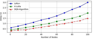
Figure 5 illustrates the relationship between network delay and the number of nodes in a LoRaWAN environment.
1. Trend Analysis: The graph typically shows that as the number of nodes increases, the delay experienced in the network also increases. This trend is indicative of the growing contention for communication resources, leading to longer wait times for packet transmission.
2. Comparison of Algorithms: The figure likely compares the delay performance of different scheduling algorithms, such as the proposed RL-based algorithm versus traditional methods like LoRa+ and RT-LoRa. The RL-based algorithm is expected to demonstrate significantly lower delays, showcasing its effectiveness in optimizing resource allocation and scheduling tasks.
3. Implications for QoS: The results presented in this figure highlight the importance of efficient scheduling in maintaining low latency, especially in scenarios with a high density of nodes. This is crucial for applications requiring real-time data transmission, emphasizing the need for advanced algorithms to manage network performance effectively.
Overall,
Figure 5 provides valuable insights into how network delay is affected by node density and the performance advantages of the proposed scheduling approach.
Figure 5. Delay vs number of nodes.
4.3.2. Packet Delivery Ratio (PDR)
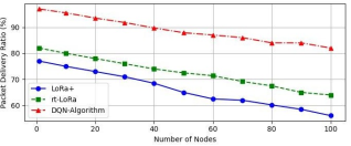
Figure 6 depicts the relationship between the Packet Delivery Ratio (PDR) and the number of nodes in a LoRaWAN network.
1. PDR Trends: The graph typically shows that as the number of nodes increases, the PDR may initially rise but eventually plateaus or declines. This behavior indicates that while more nodes can enhance network coverage, increased contention and potential collisions can negatively impact the successful delivery of packets.
2. Algorithm Comparison: The figure highlights the performance of the proposed RL-Based Algorithm (DQN) in achieving the highest PDR compared to other algorithms like RT-LoRa and LoRa+. This superiority suggests that the RL-based approach effectively manages scheduling and resource allocation, minimizing packet losses.
3. Significance for Network Performance: The PDR is a critical metric for assessing the reliability of communication in IoT networks. A higher PDR indicates better performance and reliability, which is essential for applications that require consistent data transmission, reinforcing the importance of advanced scheduling techniques in optimizing network performance.
Overall,
Figure 6 emphasizes the impact of node density on packet delivery success and showcases the advantages of the proposed algorithm in maintaining high delivery ratios.
Figure 6. Packet delivery ratio (PDR) vs Number of Nodes.
4.3.3. Packet Error Rate (PER)
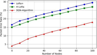
Figure 7 illustrates the relationship between Packet Error Rate (PER) and the number of nodes in a LoRaWAN network.
1. PER Trends: The graph typically shows that as the number of nodes increases, the PER tends to rise, indicating a higher percentage of packets experiencing errors during transmission. This trend reflects the increased likelihood of packet collisions and interference in a congested network environment.
2. Algorithm Performance: The figure highlights that the RL-Based Algorithm exhibits the lowest PER compared to other algorithms like RT-LoRa and LoRa+. This lower PER is attributed to the dynamic optimization of scheduling and resource allocation performed by the RL-based approach, which effectively reduces packet collisions and transmission errors.
3. Implications for Network Reliability: A lower PER is crucial for ensuring reliable communication in IoT applications, as it directly impacts the overall performance and efficiency of the network. The results presented in this figure underscore the importance of employing advanced scheduling algorithms to enhance network reliability and minimize transmission errors, especially in scenarios with a high number of nodes.
Overall,
Figure 7 emphasizes the correlation between node density and packet error rates, showcasing the effectiveness of the proposed RL-based algorithm in maintaining low error rates in a congested network.
Figure 7. Packet Error Rate (PER) vs Number of Nodes.
4.3.4. Throughput
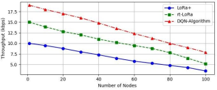
Figure 8 illustrates the relationship between throughput and the number of nodes in a LoRaWAN network. It shows that as the number of nodes increases, the throughput achieved by the RL-Based Algorithm (DQN) remains significantly higher compared to other algorithms like RT-LoRa and LoRa+. This superior performance is attributed to the RL-Based Algorithm's dynamic optimization of scheduling decisions, which effectively balances network load and minimizes collisions, resulting in enhanced data transmission rates even as node density increases.
Figure 8. Throughput vs Number of Nodes.